The BIP2 Language
Introduction
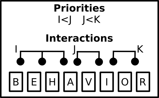
The three-layered BIP2 representation.
BIP2 (Behavior, Interaction, Priority version 2) is a component-based language for modeling and programming complex systems. In BIP2, a system is represented by:
- the behavior specified by a set of components
- a set of interactions which defines the possible synchronizations and communications between the components; they are structured in connectors that corresponds to subset of interactions (see Connectors)
- a set of priorities used for resolving conflicts between interactions or for defining interaction schedule policies (see Priorities).
With behavior, interactions and priorities we can build hierarchies of complex components called compound components or compounds for short. A compound component is composed of a set of components, connectors and priorities (see Compounds). Atomic components, or atoms for short, are the simplest component type (i.e. non hierarchical) whose behavior is expressed by automata or Petri nets (see Atoms).
In the following, we use the term component to refer to either an atomic or a compound component. The ports and variables accessible to other components and connectors define the component interface. Ports are used for component communication in a synchronized manner. Variables store information accessible to priority and transition guard expressions to resolve conflicts and non-determinism.
The BIP2 compiler processes an input file that contains a package declaration. In the processed file, a compound component, called model, describes the system we want to simulate, analyze, verify or just execute.
Quick overview of the language
Preliminary notations
In the following sections we describe the main features of the BIP2 language. The language syntax is expressed by a set of derivation rules that observe the following conventions:
- a rule begins with a name followed by the symbol ‘:=‘ and one or more terminal and non-terminal rules, e.g.: non_term := 'term' sub_non_term
- terminal elements are enclosed in ‘``’``’, e.g.: 'terminal'
Identifiers are used in many contexts to denote package names (package_name), variables (variable_name) etc. In reality, those constructs are expressed by one rule in the grammar, but for readability we refer to them with a descriptive rule synonym. You can find the full grammar in BIP 2 Grammar.
Examples of rules
sample_rule :=
  'some text' another_rule 'some ending text'

another_rule :=
  'foo bar terminal'
Annotations
Annotations offer a mechanism for defining information that are used by tools other then the compiler. The compiler examines the syntax of annotation directives but their content is ignored. BIP2 statements that accept annotations are noted by the following notation:
- accepts annotations
The syntax for the annotations is given below.
Syntax
annotation :=
  '@' annotation_name ['(' annotation_parameter (',' annotation_parameter)* ')']

annotation_parameter :=
    annotation_key
  | annotation_key '=' annotation_value
  | annotation_key '=' '"' annotation_string_value '"'
Example
@cpp(foo=bar, obj="foo.o,bar.o")
atom type MyAtom(int x)
 ...
end
Packages
A package is a unit of compilation contained in a single file. It may include other packages with the use directive. In BIP2, a package may contain:
- constant data (see Variables and data types)
- external data types (see Variables and data types)
- external functions (see Variables and data types)
- external operators (see Actions)
- port types (see Port types)
- atom types (see Atoms)
- connector types (see Connectors)
- compound types (see Compounds)
Constants are referenced in type definitions or in the initialization of other constant data. Constant data are visible only within the package that defines them.
Important
BIP2 permits the declaration of type names used for simple type checking but doesn’t support type definitions (classes, structures, etc.). It’s the responsibility of the back-ends to really interpret the types (for example, the C++ back-end will map these types to C++ types directly).
Important
To refer to types declared in other packages, prefix the type name with the name of the package where it is declared (e.g. some.pack.name.SomeAtomType)
Syntax
- accepts annotations
package_definition :=
  'package' package_name
     ('use' package_name)*

     data_type*
     (extern_function | extern_operator)*
     bip_type+
  'end'

data_type :=
 'extern data type' type_name
     [ 'refine' type_name (',' type_name)* ]
     [ 'as' '"' backend_name '"' ]

extern_function :=
 'extern function' [type_name] function_name '(' [ type_name (',' type_name)* ] ')'

extern_operator :=
 'extern oprator' [type_name] operator '(' [ type_name (',' type_name)* ] ')'
Example
package SomePackage
  const data int my_const_int = 42

  extern data type my_list

  extern function int min(int, int)
  extern function printf(string)
  extern function display(my_list)
  extern function int get(int i, my_list)

  port type Port_t()
  port type Port_t2(int i, my_list l)
end
Variables and data types
In BIP2, variables are used to store data values. Their declaration consists of a (data) type and a name. For example:
data int x
declares a variable named x of type int. The keyword data is ommited in the declaration of parameters of BIP2 types (i.e. port types, atom types, connector types, and compound types). Constant variables can also be declared in packages using the keyword const data and the initialization operator =. For example:
const data float Pi = 3.1415926
at the beginning of a package declares a constant named Pi of type float with value 3.1415926.
Important
The constant variables of packages are the only ones that can (and must) be initialized when declared. Other types of variables should be initialized after their declaration.
Types of variables are either native or external. Native types are known to the BIP2 compiler and are part of the language. Currently, the supported native types are:
- bool for boolean values false and true
- int for integers (e.g. -100, 0, 32)
- float for floating-point numbers (e.g. 2.7182818)
- string for sequences of characters (e.g. "My name is BIP2\n").
Notice that the type int is considered by the compiler as a sub-type of float regarding compatibility of types, which means each time the type float is accepted, the type int is also accepted.
Important
The exact encoding (number of bits, range) of the native data types is not specified by the semantics of BIP2. Currently, the specialization is done in the back-ends. Typically, native data types are mapped to the usual types of the target language, e.g. when using the C++ back-end the native types of bool, int, float, and string are mapped respectively to the C++ types bool, int, double, and std::string.
Notice that constant variables of packages, as well as parameters of components, can be only of a native type.
Besides the predefined native types, additional types can be declared with the keyword extern. These types are supposed to be externally defined and present when compiling the generated code. For instance, when using the C++ backend all the external types should be defined in additional C++ files included in the compilation process of the generated code. An example of declaration of an external type named IntList can be found below.
extern data type IntList refine List as "std::list<int>"
This declaration states that IntList is a valid type name. It also specifies that IntList is a sub-type of the (external) type List, and that IntList should be translated into std::list<int> by code generators (e.g. in this example we target C++ code generation). Code generators use the name of the type (in this example IntList) if the instruction as is not provided, e.g. when using the following declaration code generators will not translate IntList and use its name directly in the generated code.
extern data type IntList refine List
Important
Without any additional declation, the compiler assumes that no operation can be performed on external types except assignments (using =). This means that assignments of external types should be implemented in the generated code, e.g. by additional files included in the compilation process.
As for external types, BIP2 allows the declaration of external function prototypes that are assumed to be externally defined and present when compiling the generated code. The declaration of an external function consists of an optional return type name, a function name, and a list of types names for the arguments of the function. For example:
extern function int rand()
extern function printf(string)
extern function int getElement(int, IntList)
declares prototypes for:
- the external function rand having no argument and returning an int
- the external function printf that takes a string as argument and have no returned value
- the external function getElement that takes an int and an IntList as arguments, and returns an int.
Important
External function prototypes may involved external data types (that must be declared properly obviously). There are no specific restrictions in the declaration of prototypes concerning overloading: different prototypes may have the same function name even if they have the same number of arguments and/or different return types. This may trigger errors when compiling expressions involving calls to external functions, as explained in Actions.
Actions
Actions define computations and data transformations. In the constant context, expressions should not have side effects. Notice that the compiler is unable to check whether an external function involved in a constant context has side effects. It is the user’s responsibility to ensure the absence of side effects in such context. In the non-constant context any computation is allowed. There are also mixed contexts where some data can be changed while others can’t (see Connectors). Whenever possible, the compiler will restrict the possible actions to enforce the “const-ness”.
Computations and data transformations in actions are expressed by C-like syntax statements and expressions. Statements are assignments, function calls and conditional if-then-else constructs. Notice that the language has no support for loops. Expressions involved in statements can combine values using comparison operators, arithmetics operators, boolean operators, and function calls (with returned values). As usual, parenthesis ( and ) may be used to group expressions and enforce a specific evaluation order. Multiple statements in an action are enclosed in brackets while individual statements are separated by ;. The following operators can be used for native types.
Comparison operators can be used to compare two values of the same native type and return a value of type bool. In addition we also allow the comparison of int to float and float to int. The list of comparison operators is provided as follows.
- == : equality
- != : inequality
- < : less than
- > : greater than
- <= : less or equal than
- >= : greater or equal than
Arithmetic operators provided below can only be applied to numbers, i.e. int and float data types. They return a value of type int if all the arguments are of type int. They return a value of type float otherwise.
- / : division
- % : modulo
- + : addition or positive sign
- - : subtraction or negative sign
- * : multiplication
Logical boolean operators apply to boolean values only (of type bool), and return boolean values:
- && : logical and
- || : logical or
Boolean bitwise operators apply to int only, and return int:
- & : bitwise and
- | : bitwise or
- ^ : bitwise exclusive or
- ~ : bitwise not
- ! : logical not
The assignment operator may assign a value to a variable provided that the type of this value is compatible with the type of the variable, that is, if it is of the same type or if it is of a sub-type. Notice that in contrast to previous operators, by default the assignment operator applies also to external types.
- = : assignment
Important
The exact behavior data types and corresponding operations is not specified by the semantics (e.g. min/max ranges of integer and floating point types, behavior of overflows, etc.). Currently, the specialization is done in the back-ends (usually by mapping directly BIP2 types and operations to usual types and operations of the target language).
In addition to the predefined operators, external functions can be call provided their prototype is declared, as explained in Variables and data types. We say that a function call matches a prototype if it has the same function name and the same number of arguments, and if its arguments are compatible with the ones of the prototype. We say that a prototype is strictly more precise than another prototype if it has compatible arguments with at least one being a strict sub-type. For example in the following the first prototype is strictly more precise than the third prototype, whereas it is not comparable with the second prototype:
extern function float min(float, int)
extern function float min(int,   float)
extern function int   min(int,   int)
A function call will not compile if one of the following assertions apply:
- it does not match any declared external function prototype (“no match prototype” error)
- it matches at least two prototypes without one beging strictly more precise than the other one (“ambiguous function call” error)
- the return type of the most precise matching prototype is not compatible with the rest of the expression in which the function is called (“incorrect type” error)
- the most precise matching prototype has no return type and the function call is involved in an expression (“no return value” error).
Considering that the prototypes for min are restricted to the following:
extern function float min(float, int)
extern function float min(int,   float)
then the statement x = min(0, 0); will lead to a compilation error such as:
[SEVERE] In /path/to/file/my_bip_file.bip:
Ambiguous function call 'min' with parameter(s) of type(s) 'int, int': cannot decide
between 'float min(float, int), float min(int, float)' :
    38:
    39:         x = min(0, 0);
--------------------^
    40:
    41:
Similarly to external functions, external operators can be declared by using extern operator followed a return type, the target operator (instead of the function name) and its arguments, e.g.:
extern operator string +(string, string)
These declarations should always include a return type, and are limited to the number of arguments a given operator has in the language for native types. For example, in the following code the first two declarations are not permitted whereas the last two ones are accepted:
extern operator Complex *(Complex)           // not valid: missing argument    - ERROR!
extern operator         *(Complex, Complex)  // not valid: missing return type - ERROR!
extern operator Complex *(Complex, Complex)  // OK
extern operator Complex *(float,   Complex)  // OK
Notice that declarations of external comparison operators (==, !=, <, >, <=, >=) are not forced to return boolean values, but for readability of the code we recommend to avoid such practice. Similarly, logical operators (!, ||, &&) may be redefined for non boolean values, but again we strongly recommend not doing it:
extern operator int     ==(IntList, IntList)  // allowed but not recommended!
extern operator IntList ||(IntList, IntList)  // allowed but not recommended!
Example
{
  a = a * (2 + b);
  g(d);
  b = f(a);
}
In a constant context, an action contains a single expressions enclosed in parenthesis that must evaluate to a boolean value.
Important
Depending on the locations of the actions, the data reference can take different forms. For example, in Atoms, the data can be directly referenced by its declaration name whereas a connector action referencing a data within a port must use a dotted notation (e.g. port_name.data_name).
There is currently only one control flow operation: if-then-else with the following syntax:
if ( boolean_condition ) then
  statement1;
else
  statement2;
fi
The else part is optional and may be omitted. The expression boolean_condition must evaluate to a boolean value.
Port types
Ports are used to synchronize component and convey information in a synchronized manner between the components of a model. The transferred information is accessible via the variables associated with the port. Port types are declared with the port type keyword followed by the port type name and a possibly empty list of accessible variables. The following example declares a port with type port_t which can access integer values from the x variable:
port type port_t(int x)
Syntax
- accepts annotations
port_type_definition :=
  'port type' (package_name '.')? port_type_name
    '(' data_param_declaration (',' data_param_declaration)* ')'
Atoms
Atoms are the simplest components with a behavior described by an automaton or a Petri net extended with data. An atom type is declared with the atom type directive which contains:
- a possibly empty list of variables for storing data. Data declarations may be exported to become accessible to priorities.
- an optional list of port declarations that may reference variables. Exported ports are accessible to connectors.
- an automaton or a Petri net that defines the behavior of the atom. The behavior is described by a set of transitions that change the state of the atom in reaction to enabled ports.
Data types and variables
- In BIP2, (data) variables are used to store data. A declaration of a variable is
data keyword. For example:
data int x
declares an integer variable named x.
Variables exported with the export directive can be used in guards of compound component priorities (see Compounds).
Ports
Atoms have ports declared with the port directive that consists of a type, a name and an optional list of previously declared variables. It is an error if the types of the previously declared variables do not match the type of the corresponding port parameters. Implicit type casting is not permitted. For example, if a previously declared parameter is of type float, a port parameter of type int is not allowed. In the following code excerpt, three variables named a, b and c are associated with the three parameters of the port with type Port_t:
port type Port_t(int x, float y, some_type z)

atom type SomeType()
  data int a
  data float b
  data some_type c

  port Port_t p(a, b, c)
  ...
end
Ports can be exported with the export directive and become accessible to other model components. Exported ports can be accessed individually in the component interface (see Figure 2.2) or merged into one port (see Figure 2.3). In the later case, they must accept the same number and types of parameters. The merged port provides access to all variables of the individual ports.
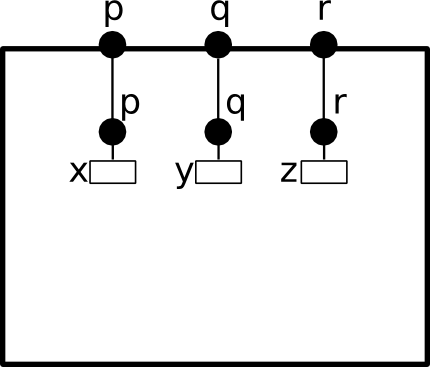
Ports p, q and r are individually exported.
In BIP2, ports p, q and r are individually exported using the following statement:
export port port_t p(x), q(y), r(z)
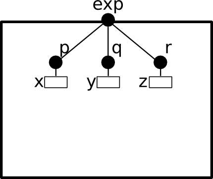
Ports p, q and r are merged and exported as the port exp.
To merge and export ports p, q and r as a single port exp we use the keyword as:
export port port_t p(x), q(y), r(z) as exp
Petri net
Petri nets implement the behavior of atoms. They consist of places and transitions. Places are used to store the current control location of the atom given by a marking of the places, that is, a boolean function associating true to the marked places. Places are declared in an atom using the keyword places followed by a list of place names, e.g. the following code declares the places named START, SYNC and END:
places START, SYNC, END
Transitions change the current state of an atom and invoke associated actions that may alter the values of atom variables. A transition specifies:
- The set of triggering places that are required to be all marked at the current state for the transition to occur. They are declared using the keyword from.
- The set of target places that are marked after its execution. They are declared using the keyword to.
- A boolean condition on values of (local) variables that must be fulfilled at the current state for the transition to occur. This condition, called guard, is declared using the keyword provided. If no expression is provided, the guard places no restrictions on the transition.
- An optional block of code after the do keyword that is evaluated when the transition occurs.
A transition of an atom is enabled if:
- it is enabled by the marking, that is, all its triggering places are marked at the current state and
- the associated guard evaluates to true or there is no guard associated with the transition.
Important
Notice that in BIP2 we target 1-safe Petri nets where the target places of an enabled transition are never marked. This property for a Petri net of an atom is checked both at compile time and at run time, and leads to an error if violated. Notice that since automata are a sub-case of 1-safe Petri nets, they can be used to define the behavior of atoms. In automata, each transition has at most one triggering place and one target place.
We distinguish three types of transitions:
The initial transition is responsible for initializing the marked places and atom variables. It is a mandatory transition executed once during the model initialization. It has no triggering places and no associated guard. Moreover, the initial transition can not be observed by other components nor synchronized with their transitions. For example, the following code fragment specifies the initial transition of an atom that marks the place START and initializes the variables x and y:
initial to START do { x=0; y=0; }Internal transitions are invisible to other components and take precedence over other observable transitions. Their execution depends on the current state and associated guards. Internal transitions are declared using the keyword internal, e.g. the following specifies an internal transition enabled in the START place that sets the current state to the SYNC place restricted by an associated guard:
internal from START to SYNC provided (x!=0) do { x=f(); }Transitions labeled by internal port names are visible to other components. A transition labeled by an internal port that is exported can be synchronized with transitions of other components using connectors (see _language-connector-label). Such transitions are declared in atoms using the keyword on, e.g. the following specifies a transition labeled by the internal port s, that changes the current state from SYNC to END:
on s from SYNC to END
The following figure gives an example of execution sequence of transitions in an atom A in which the initial transition is followed by the execution of an internal transition, then a transition labeled by port p is executed followed by the execution of two internal transitions, and finally a transition labeled by port q is executed leading to a state in which no transition is enabled. Notice that the only visible states of A are the ones preceding the executions of p and q and the final state, the other intermediate states are invisible.
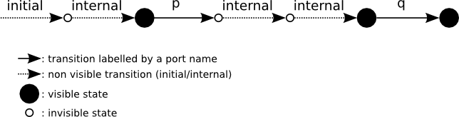
Sequence of internal and visible transitions in an atom.
Important
Only one internal transition is enabled at any time since non-determinism is not allowed for internal transitions of atoms. Similarly, two transitions labeled by the same internal port name must not be enabled at the same time.
Priorities
Priorities are used to resolve conflicts or to define an ordering between transitions labelled by ports: the selected transition corresponds to the port with highest priority. They may also include a boolean expression called guard that specifies the conditions when it is applicable. Priorities do not apply to the initial and internal transitions. In the following example, port q has higher priority than p provided that variable x equals to zero.:
priority myPrio p < q provided (x==0)
The transitive closure of such priorities defined in an atom is a partial order relationship among ports and associated transitions. A port q has higher priority than p if there is a priority rule specifying p < q whose guard evaluates to true, or there are ports p1, p2, ..., pN such as p < p1 < p2 < ... < pN < q such that all their corresponding guards evaluates to true. Notice that it is not required for ports p1 to pN to be enabled. An enabled transition is maximal if it has the highest priority.
Important
Inconsistencies in priorities (e.g. a < b < c < a) are detected and reported. If the priorities do not include guards, the checks are performed at compile time. Guard expressions can not be evaluated during the model compilation so in this case priority validation is postponed until run time.
Enabled ports of atoms
An internal port is enabled if it triggers an enabled transition for the current atom state. The port is maximal if its corresponding enabled transition is maximal. An exported maximal port is also enabled at the interface level. When several maximal internal ports are exported through the same port (i.e. merged export), they are all visible to other components that can interact with any of the internal ports through the interface. Consequently, if an internal port references variables, the values accessible from the interface are the values of the enabled maximal internal ports.
The following figure illustrates an example of a merged port named exp that consists of three internal ports p, q and r and each internal port references a variable (e.g. x, y and z). Port exp is enabled if at least one of the corresponding ports is enabled. However, only the variables of the enabled internal ports are accessible from the interface. For example, if ports x and z are enabled, the associated u and w values are accessible from exp. On the other hand, if only port y is enabled, the value associated with port exp is v. This means that when other components interact with A through port exp, depending on which of the internal ports is enabled, they interact with port p using value u, or with port q using value v, or with port r using value w.

Example of a port enabled by an atom and the corresponding values of its variable.
Example
atom type MyAtom(int P)
         data int x
  export data int y

         port Port_t r(x), s(y)

  places START, SYNC, END

  initial             to START                do { x=P; y=0; }
  internal from START to SYNC provided (x!=0) do { y=f(x); }
  on r     from START to SYNC                 do { y=x; }
  on s     from SYNC  to END
end
The above block of BIP2 code gives an example of atom type MyAtom that accepts one integer parameter P, and consists of two integer variables x and the exported variable y and two exported ports r and s. Three places, START, SYNC, END, are the states of the automaton that defines the behavior of the atomic component. An initial transition leads to START, an internal transition changes the state from START to SYNC, an other transition triggered by r does the same and finally a transition triggered by s modifies the state from SYNC to END. A graphical representation of MyAtom is provided below.
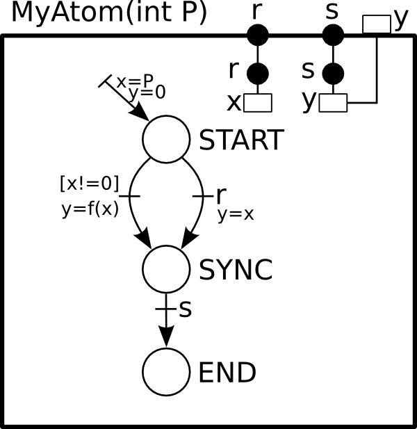
Since internal transitions have higher priority than port transitions, the transition of port r is executed only if the guard of the internal transition does not hold, i.e. the value of variable x is zero.
Syntax
- accepts annotations
atom_type_definition :=
  'atom type' atom_type_name '(' [ data_parameter (',' data_parameter)* ] ')'
     (['export'] 'data' data_type
        data_declaration_name ( ',' data_declaration_name )* )*
     (['export'] 'port' port_type
        port_name '(' data_declaration_name (',' data_declaration_name )*) ')'
        ( ',' port_name '(' data_declaration_name (',' data_declaration_name )*) ')' )*
        ['as' port_name] )*
     'place' place_name (',' place_name)*
     'initial to' place_name (',' place_name)* ['do' actions]
     ( ('on' port_name | 'internal')
        'from' place_name (',' place_name)*
        'to' place_name (',' place_name)*
        ['provided' '(' transition_guard ')'] )*
        ['do' actions]
     atom_priority_declaration*
   'end'
Connectors
Connectors are stateless entities that enable interactions among a set of components via their interface ports. Interactions defined by a connector are strong synchronizations (i.e. a rendez-vous) of a subset of the connected components. Interactions may also include data that are transferred between the components. A connector is hierarchical if it connects ports exported by other connectors.
Connected ports
A connector type accepts a list of typed ports that correspond to the ports of the entities it connects (components or other connectors). Connectors (i.e. instances of connector types) bind these parameters to actual ports of the same type.
Important
Components or connectors must be connected at most once in a connector, that is, a component or a connector must not be reachable from different connected ports.
Data variables
Connector types can define variables that are used for storing intermediate results of computations performed in transfer functions associated with interactions. The temporary stored value is accessible only during the associated interaction. The syntax is shown in the following example where we declare an integer variable named tmp:
data int tmp
Exported port
A connector may export a single port that can be connected to other connector instances and form hierarchical connectors, or it can be exported in the interface of compound components (see Compounds). A connector is top-level if the exported port is not connected directly to another connector (i.e. it can be connected to other connectors only at upper levels after being exported by the containing compound), or if it has no exported port. An exported port named exp of type port_t, referencing a variable tmp, is declared in a connector type as follows:
export port port_t exp(tmp)
Defined interactions
Formally, an interaction of a connector type is a subset of its ports. A connector type explicitly define a set of permitted interactions regardless of the status of the connected ports. The interactions are defined in terms of expressions involving port names, according to the following grammar:
connector_port_expression :=
  ( sub_expression )+

sub_expression :=
  ( port_name | '(' connector_port_expression ')' ) [''']
That is, an expression is a list of either port names or nested expressions (expressions enclosed into parenthesis) that can be optionally quoted. Quoted port names or nested expressions are called triggers, whereas unquoted ones are synchrons.
An expression of the form p, where p is a port name, defines a single interaction ‘p‘. Interactions defined by an expression of the form e' are the ones defined by e. Interactions defined by an expression of the form e1 e2...eN are computed recursively from the interactions defined by sub-expressions e1, e2, ..., eN, as explained as follows. An interaction is defined by e1 e2...eN if both following rules apply:
- it can be written as a union of interactions defined by sub-expressions e1, e2, ..., eN
- it contains (at least) an interaction defined by a trigger sub-expression, or for each sub-expression eI, I=0,...,N, it contains an interaction defined by eI.
In the following example we define one trigger sub-expression (p q), and two synchrons ports r and s:
define (p q)' r s
Interactions permitted by such an expression are the ones containing (at least) both ports p and q, i.e. ‘p,q‘, ‘p,q,r‘, ‘p,q,s‘ and ‘p,q,r,s‘.
Guards and transfer functions
The set of defined interactions in a connector type can be further restricted by guards. Guards evaluate a boolean expression that refers to variables of the ports involved in an interaction. The associated interaction is enabled only if the guard evaluates to true.
Transfer functions are used for exchanging data between the components that participate in an interaction. They consist of two instruction groups, the up and the down group.
The up instructions compute the values of the variables referenced by exported ports. Also, intermediate values used in computations in the down section may be temporary stored in the connector’s variables. In the following example we define a rendez-vous interaction between two ports where a temporary value is stored in the tmp variable. To prevent division by zero, the interaction is disabled when the value of the y variable equals 0:
on p q provided (q.y != 0) up { tmp = p.x / q.y; }
The down instructions may update the values of the variables associated with the ports involved in an interaction. Port variables are assigned with values computed from connector variables and variables of the exported port. In the following example, the instructions swap the values of variables x and y of ports p and q:
on p q down { tmp = p.x; p.x = q.y; q.y = tmp; }
Notice that transfer functions up and down can be simultaneously defined for a connector interaction. up functions correspond to data moving upwards in the connector and component hierarchy, that is, from values of variables of the connected ports to the values of variables of the port exported by a connector. Once an interaction is chosen and executed, down functions correspond to the downward flow of data, that is, from variables of the exported port to variables of the connected ports.
Important
For a given interaction, the temporary values of connector variables when executing the down instructions are computed by the corresponding up instructions. However, these values are not accessible between different executions of the same interaction or between the execution of the transfer functions of different interactions. They are only stored between the execution of up and down instructions of the same interaction.
Example
connector type ConnectT(Port_t1 p, Port_t2 q, Port_t3 r)
  data int tmp
  export port Port_t exp(tmp)

  define p' q r

  on p     up { tmp = p.x; }                down { p.x = tmp; }
  on p q   up { tmp = max(p.x, q.y); }      down { p.x = tmp; q.y = tmp; }
  on p r   up { tmp = max(p.x, r.z); }      down { p.x = tmp; r.z = tmp; }
  on p q r up { tmp = max(p.x, p.x, r.z); } down { p.x = tmp; q.y = tmp; r.z = tmp; }
end
In the previous BIP2 code excerpt we provided a complete definition of a connector type named ConnectT that connects three ports p, q and r. We have already seen in previous examples the enabled interactions and the computations performed by the transfer functions. A noticeable difference is that variable tmp is accessible to other connectors that interact with port exp. Hence, the value of tmp may differ from the computation performed by up since it may be altered by the transfer functions of connectors connected to exp. A simplified graphical representation of ConnectT is provided below.
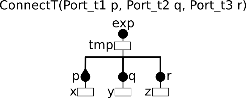
Connector type example
Enabled interactions and ports exported by connectors
The set of ports defined by an interaction is restricted at run time based on the status of the involved ports and the evaluated guards. Let us consider an example of interaction involving ports p, q and r:
define p' q r
Based on the definition above, the permitted interactions are (‘p‘, ‘p,q‘, ‘p,r‘ and ‘p,q,r‘). To determine which of the combinations are valid in a model execution, we first remove all combinations that contain a disabled port and then we evaluate the associated guards to further restrict the possible combinations.
An exported port of a connector is enabled if there is at least one enabled interaction. Notice that the value visible at the interface through the exported port is derived by the set of values of ports participating in an interaction. The values accessible from an enabled interaction are in turn computed by the instructions of the up transfer function.
The notions of enabled interactions and corresponding values of the variables of exported ports of connectors are illustrated by the following example. Consider an instance C of the connector type ConnectT presented above. Assume that ports p, q, r are enabled, and that variable x of port p has three possible values u1, u2, u3, variable y of port q has three possible values v1, v2, v3, and variable z of port r has only a single value w. Then, interactions ‘p‘, ‘p,q‘, ‘p,r‘ and ‘p,q,r‘ are enabled. Moreover, there are 24 possible values for variable tmp of the exported port exp, corresponding to the application of up to all combinations of values for the 4 enabled interactions:
- The values corresponding to interaction p are the values of x, that is, u1, u2 and u3.
- The values corresponding to interaction p,q are oIJ- = max(uI, vJ), such that I=1,2,3 and J=1,2,3.
- The values corresponding to interaction p,r are oI-* = max(uI, w), such that I=1,2,3.
- The values corresponding to interaction p,q,r are oIJ* = max(uI, vJ, w), such that I=1,2,3 and J=1,2,3.
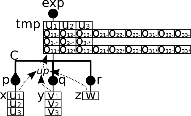
Enabled interaction of a connector and the corresponding values of variable tmp.
Syntax
- accepts annotations
connector_type_definition :=
  'connector type' connector_type_name '(' port_parameter (',' port_parameter )* ')'
    ('data' data_type data_declaration_name ( ',' data_declaration_name )* )*
    ['export port' port_type
       port_name '(' data_param_declaration (',' data_param_declaration)* ')' ]
    'define' connector_port_expression
    connector_interaction*
  'end'

connector_interaction :=
  'on' (port_name)+
  ['provided' '(' connector_guard ')']
  ['up' '{' (statement ';')+ '}']
  ['down' '{' (statement ';')+ '}']

connector_port_expression :=
  ( port_name ['''] | '(' connector_port_expression ')' ['''] )+

(a connector interaction must have at least one of 'up', 'down' or 'provided')
Compounds
Compounds are composite components constructed by atomic components and other compound components. Just like atomic components, compounds provide a set of ports at the interface level. In this sense, components are used in the same way regardless of their structure (compounds or atomic). A compound type defines the following.
a set of components, either atomic or compound, declared with the keyword component.
a set of connectors declared with the keyword connector that connect the contained components.
a set of priority rules declared with the keyword priority.
- a set of exported ports that define the interface of the compound declared
with the keyword export.
Notice that a compound component can export ports of contained components as well as ports of connectors.
Priorities
Priorities are used to favor the execution of a subset of enabled interactions called the maximal interactions (see below for a definition of maximal interactions). They can be used to resolve conflict between interactions or to express particular scheduling policies.
Priorities of a compound, form a partial order relationship that corresponds to the transitive closure of the defined priority rules. One set of priority rules is automatically derived based on the maximal progress principle, i.e. interactions that involve more connectors have higher priority.
User-defined priority rules are of the form I < J, where I and J are interactions of connectors expressed in one of the following forms:
- C:A1.p1,A2.p2,...,AN.pN where C is a connector and A1.p1,A2.p2,...,AN.pN is a subset of the connected ports that corresponds to a defined interaction of C.
- C:*, where C is a connector represents all the defined interactions of C.
- *:* represents all the defined interactions for all connectors.
Important
User-defined priority rules can only involve interactions of top-level connectors.
The use of * in priority rules is a shortcut for sets of rules. Notice that *:* cannot be used for both sides of a priority rule, (e.g. *:* < *:* is not allowed). The use of *:* in one side of a priority rule is a shortcut for all interactions defined in all connectors except those involved in the other side of the rule.
User-defined priority rules may include guards declared with the provided keyword. A rule is enabled only if its guard evaluates to true. In the following code excerpt we show a priority rule named myPrio that is enabled only if the values of the x and y variables of the atomic components A and B are not the same:
compound type Compound_T()
  component Atom_T A()
  component Atom_T B()

  connector RDV C(A.p,B.p)
  connector RDV D(A.q,B.q)

  priority myPrio provided (A.x != B.x) C:A.p,B.p < D:A.q,B.q
end
Important
Since priorities define a partial order relationship between interactions, priority rules enabled at a state of a compound must not form a cycle.
An enabled interaction I of a connector C has lower priority than an enabled interaction J of a connector D if D is reachable from I in the lattice of the defined priority rules, that is, if C:I < D:I is an enabled rule or if there exists interactions C1:I1, ..., CN:IN such that rules C:I < C1:I1, C1:I1 < C2:I2, ..., CN-1:IN-1 < CN:IN, CN:IN < D:J are enabled. An interaction is maximal if it has the highest priority among the enabled interactions.
Exported ports and variables
Compound types export ports and variables in a similar fashion with atoms . The following statement makes the x variable accessible from the interface of the A component and renames it to y:
export A.x as y
Ports of components and connectors can be exported individually or through a single port using a merged export, in the same way as atoms. To determine if a port of a compound component is enabled we check if the underlying port (component or connector port) is enabled. If a port of a component is enabled and exported, then the corresponding port at the interface is enabled. If a (maximal) interaction is enabled in a connector that exports its port to the interface of a compound, then the interface port is enabled. Moreover, values visible at the interface are the values corresponding to all its maximal interactions. As for atoms, for merged exported ports the union of the values is visible at the interface.
compound type Compound_t()
  component Atom_t      A(), B()
  connector Connector_t C1(A.p, B.p)
  connector Connector_t C2(A.q, B.q)

  export C1.exp, A.r, B.r as s

  priority myPrio C1:A.p,B.p < C2:*
end
In the above example, the port s of an instance of the compound type Compound_t is enabled if the connector C1 has a maximal interaction (i.e. if no interaction is enabled by C2), or if port r of A is enabled, or if port r of B is enabled. Moreover, if these ports have variables, the values visible from s are the union of the values corresponding to the maximal interactions of C1 and the values visible from ports r of A and B.
Example
compound type Compound_t()
  component CompT1 K1()
  component CompT2 K2()
  component CompT3 K3()

  connector BRDXP C(K1.p, K2.q)
  connector RDVXP D(C.xp, K3.t)
  connector RDV   E(K2.q, K3.s)

  export port C.xp as u
  export port F.xp as v
  export port K3.t as w

  export data K3.x as x
end
The above example shows the syntax for defining a compound type Compound_t that consists of:
- the components K1, K2 and K3
- the connectors C, D and E, such that C and D are connected and form a hierarchical connector
- the exported ports xp of C and F and the exported port t of K3
- the exported variable x of K3.
A graphical representation of the compound type is provided below. Notice that all the enabled interactions of connector C are visible from connector D through the port xp of C, e.g. if p and p,q are enabled, there are both visible from D. Since priorities are applied when exporting ports to the interface of a compound, only maximal interactions of C are visible from the interface port u though xp, e.g. if interaction p and p,q are enabled, only p,q is visible from u due to the default priority rule of maximal progress: p < p,q. Notice also that a port can be connected to several connectors (e.g. port q of K2), or can be exported and connected to connector(s) (e.g. ports xp of C and t of K3).
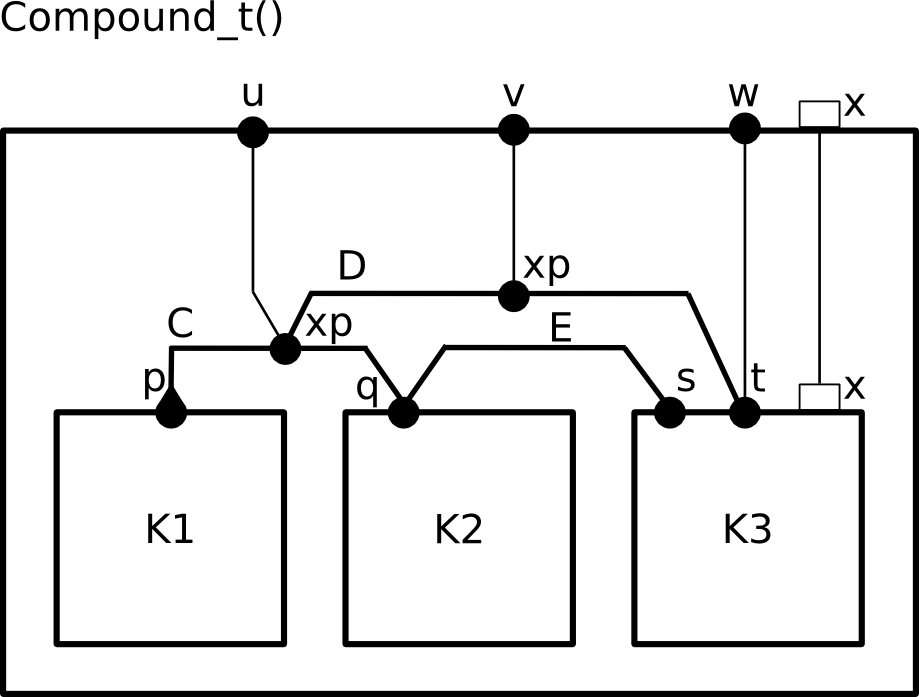
Example of a compound type.
Syntax
- accepts annotations
compound_type :=
  'compound type' compound_type_name '(' [data_parameter (',' data_parameter)*] ')'
    component_declaration+
    connector_declaration*
    compound_priority_declaration*
    inner_port_export*
    inner_data_export*
  'end'

inner_port_export :=
  'export port' port_reference (',' port_reference)* 'as' exported_name

inner_data_export :=
  'export data' data_reference 'as' exported_name

compound_priority_declaration :=
  'priority' priority_name
      ('*:*' | compound_interaction) '<' ('*:*' | compound_interaction)
      [ 'provided' compound_priority_guard ]

compound_interaction :=
  connector_name ':' ('*' | (port_reference (',' port_reference)*))
Execution sequences
A BIP2 model is equivalent to a labeled transition system (LTS) that defines all the allowed execution sequences. The model state is stored in the state of atomic components represented by variable values and the marking of the Petri nets. An execution sequence is a sequence of transitions or interactions that modify the global state. The transitions and interactions that are available in a certain state are defined as follows.
- A transition of an atom A is executed from a state if it is enabled, is maximal and is not labeled by an exported internal port.
- An interaction of a connector C is executed if it is enabled, is maximal and connector C does not export a port.
In a given state, only the non exported maximal transitions and interactions are allowed. During their execution, non maximal exported transitions or interactions are executed according to the hierarchy of connectors in the model.
The execution of an enabled transition modifies the current state as follows:
- marking of Petri nets are modified according to the triggering and target places of transitions, i.e. marks are removed from triggering places and are set in target places
- variables are modified by the code associated with the transition.
Important
If a place is both a triggering and a target place for a transition, its mark remains unchanged.
An interaction ‘p1,p2,...,pN‘ of a connector C, considering a particular combination of values for its ports, modifies the model state as follows.
First, the instructions associated with the down transfer function are performed for the values of the involved ports p1, ..., pN. Then, the state is modified according to the execution of ports p1, ..., pN.
- The execution of an atom port is equivalent to the corresponding transition.
- The execution of a compound port corresponds to the execution of the corresponding port.
- The execution of a connector port corresponds to the execution of the corresponding interaction.
Important
The execution of an interaction corresponds to the execution of at most one transition of each atom of the model. Since atoms have disjoint sets of variables and places, the state of the model resulting from the execution of an interaction is independent from the order of execution of the involved atoms.